In addition to presenting a physically important system, this lecture, reveals a very deep connection which is at the heart of modern applications of quantum mechanics. We will see that the quantum theory of a collection of particles can be recast as a theory of a field (that is an object that takes on values at every point in space). You are all familiar with classical field theories -- one example is the wave equation. Another example is the Schrodinger equation. This is part of wave-particle duality: the theory of a single quantum particle is the classical theory of a wave (plus some rules about how measurement works).
This approach is ubiquitous. For example, a common way to understanding high energy physics phenomena is to write down a classical field theory with the same symmetries then ``quantize" it using techniques like those you will learn in this lecture. On the other hand, a common approach in condensed matter physics involves having a complicated microscopic model of interacting constituents, then extracting an effective low energy field theory. In both areas, the techniques of quantum field theory are also general-purpose tools for calculating things.
In this lecture we will start with a discrete approximation to a classical field theory (a varient of an elastic rod), quantize it, and show that it can be recast as a theory of particles. These emergent particles are referred to as phonons -- quanta of sound. The same sort of arguments connect classical light waves, and photons. Of course, since Maxwell's equations are a bit more complicated than the wave equation, the theory of photons is a bit more complicated (not much though).
This is a fairly sophisticated story -- so it will essentially take me two lectures to complete it.
Before proceeding with our model, it is useful to review a few features of classical sound in real materials. A typical mental model is that we have a bunch of ball connected by springs:
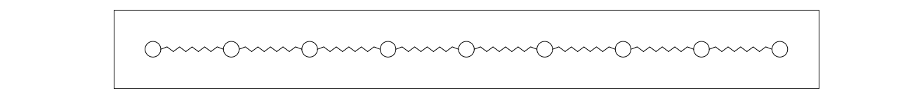
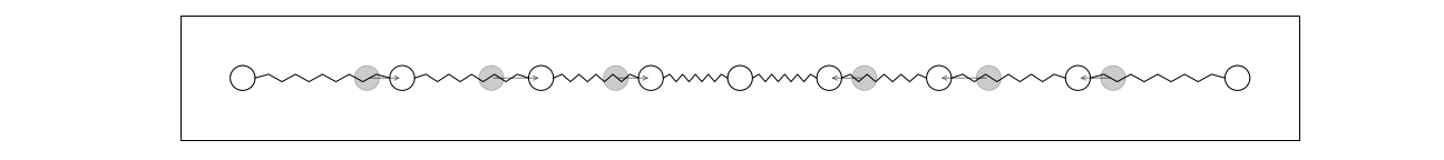
This will have two types of sound waves: longitudinal modes, where the atoms move in the direction of propegation:
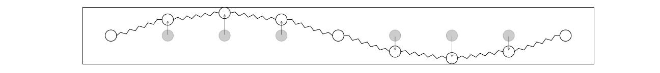
and transverse modes, where the atoms move perpendicular to the direction of motion:
For concreteness we will think about longitudinal modes, though (as you know from PHYS 2214/2218) the theory of transverse sound is pretty similar. I do, however, want to add one more level of sophistication. Most materials have more than one type of atom. Thus our model should really have at least two different types of balls:
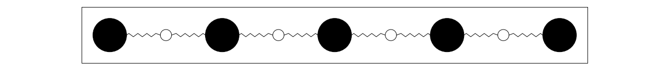
In these more complicated materials there will be ``acoustic modes," where all of the atoms move together, and ``optical modes" where the black and white atoms move out of phase. These latter modes are known as ``optical" because generally they involve a finite time-dependent polarization -- and hence can couple to light. All of these can be either longitudinal or transverse (so you will hear people talking about longitudinal optical modes, or transverse optical modes,...] We are going to make a toy model of the longitudinal acoustic modes. We imagine that the heavy atoms are essentially stationary, and only the light atoms move. There will be a weak coupling between the light atoms, yielding a model something like:
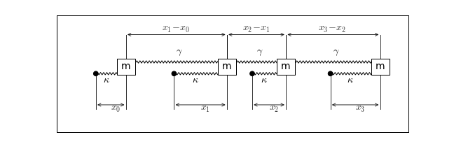
We have added labels to show that the $j$'th particle is displaced by a distance $x_j$ from its equilibrium position (at position $j*a$, where $a$ is the "lattice constant"). It feels a restoring force with spring constant $\kappa$ -- representing the coupling with the heavy atoms. The $j$'th particle will also be attached by a spring to the $j+1$'th particle. These springs will have spring constant $\gamma\ll\kappa$. We want a quantum description of this system. We start by writing the classical energy \begin{equation}\label{energy} E=\sum_j \frac{p_j^2}{2m} + \frac{\kappa}{2} x_j^2+\frac{\gamma}{2} (x_j-x_{j-1})^2. \end{equation} The quantum mechanical version of this just requires taking $p_j\to-i\partial_{x_j}$, and using this in a big Schrodinger equation $H\psi(x_1,x_2,\cdots,x_N)=E\psi(x_1,x_2,\cdots,x_N).$ Although it might seem hard to believe, it turns out we can exactly solve this model. In the spirit of this course, however, I am going to show you an approximate method which will give us a bit more insight. The approximation is going to rely on the fact that $\gamma\ll\kappa$. The first step of this approximation is a little abstract. I am going to introduce smeared out ``ladder operators" for the $j$'th particle. Since the $j$'th particle is coupled to the $j\pm1$'th particles, the appropriate ladder operators should somehow involve all three particles. In fact, in the general case the operators involve all the particles. To lowest order in $\gamma/\kappa$ it suffices to include only the nearest neighbors. I'll explain how I got this later, but what I am going to do is guess \begin{eqnarray}\label{can} x_j &=& \frac{d}{\sqrt{2}} \left([(a_j+a_j^\dagger)+ \alpha(a_{j+1}+a_{j+1}^\dagger+a_{j-1}+a_{j-1}^\dagger)\right]\\ p_j &=& \frac{\hbar}{\sqrt{2} d i} \left([(a_j-a_j^\dagger)- \alpha(a_{j+1}-a_{j+1}^\dagger+a_{j-1}-a_{j-1}^\dagger)\right], \end{eqnarray} where $\alpha$ is supposed to be small [ie. of order $\gamma/\kappa$]. The parameters $d$ and $\alpha$ will be set later. If we take $\alpha=0$, and $d^4=\sqrt{\hbar^2/m\kappa}$ this is just the standard definition of ladder operators. Even with $\alpha\neq0$ these can be ladder operators for independent harmonic oscillators, if we can arrange \begin{eqnarray}\label{com} [a_i,a_j]&=&0\\ { [a_i,a_j^\dagger]}&=&\delta_{ij} \end{eqnarray} Lets assume that equations~(\ref{com}) are satisfied. We then need to verify that the $x$'s and $p$'s have the right commutation relations: \begin{eqnarray}\label{xcom} [x_i,x_j]&=&0\\\label{pcom} [p_i,p_j]&=&0\\\label{xpcom} [x_i,p_j]&=&i\hbar \delta_{ij} \end{eqnarray} where $\delta_{ij}$ is the Kronecker delta, equal to zero if $i\neq j$ and 1 if $i=j$. The first two relations Eqs.~(\ref{xcom}) and (\ref{pcom}) are "trivially" satisfied since $[a_i+a_i^\dagger,a_j+a_j^\dagger]=0$ and $[a_i-a_i^\dagger,a_j-a_j^\dagger]=0$. The last relationship needs more work. The only cases that need to be considered are the one with $i=j$ and the one with $i=j+1$. Lets start with $i=j$. Doing the commutator term by term gives \begin{equation} [x_i,p_i]=i\hbar(1-\alpha^2). \end{equation} This is good enough for me. If $\alpha$ is small, then $\alpha^2$ is really small. Of course, it wouldn't be too hard to modify our ansatz to get rid of this small discrepency. It would probably make future book-keeping a bit harder though. A good rule of thumb is don't use a more accurate model/approximation than you have to. You often learn more from the cruder approach. Now lets look at the nearest neighbor term. There we get \begin{equation} [x_i,p_{i+1}]=\frac{\hbar}{2i} \left([(a_i+a_i^\dagger,-\alpha (a_i-a_i^\dagger)]+[\alpha(a_{i+1}+a_{i+1}^\dagger),a_{i+1}-a_{i+1}^\dagger]\right). \end{equation} The two terms in parenthesis are clearly the negative of one-another, so we get $0$, as desired. We now substitute our ansatz in Eq.~(\ref{com}) into our Hamiltonian in Eq.~(\ref{energy}). If we are not careful things will get messy. Rather than just blindly jumping in, it is useful to write the form that expression will take: \begin{eqnarray} H&=&\sum_j \left[ \left(\frac{\hbar\omega_0}{2} +t\right) (a_j^\dagger a_j +a_j a_j^\dagger) -t (a_{j+1}^\dagger a_j+a_j^\dagger a_{j+1}) \right. \\\nonumber&&\quad \left. \phantom{\frac{1}{2}} + \Delta_0 (a_j a_j+a_j^\dagger a_j^\dagger)+\Delta_1(a_j a_{j+1}+ a_{j+1}^\dagger a_j)+\cdots \right], \end{eqnarray} here $\omega_0, t, \Delta_0,$ and $\Delta_1$ are all functions of $m, \kappa, \gamma,$ and $\alpha$. The neglected terms are all of order $(\gamma/\kappa)^2$, so we can ignore them. The cool thing is, that if we know what the form is, we can ask what each of these coefficients is -- one by one. The resulting expressions are going to be a lot less messy. This is a good general strategy. In your homework you will calculate these terms -- and you will find that you are able to choose $\alpha$ and $d$ such that $\Delta_0=\Delta_1=0$. With that choice, the theory is described by the Hamiltonian \begin{eqnarray} H&=&\sum_j \left[ \left(\frac{\hbar\omega_0}{2} +t\right) (a_j^\dagger a_j +a_j a_j^\dagger) -t (a_{j+1}^\dagger a_j+a_j^\dagger a_{j+1}) \right]. \end{eqnarray} This is an interesting expression, as it has one important symmetry: the number of "quanta" are conserved. That is $N=\sum_k a_j^\dagger a_j$ commutes with the Hamiltonian, and $N$ is therefore a constant of motion. Lets specialize to the case $N=1$. The Hilbert space for this sector is spanned by the states $|j\rangle$ -- defined to be the state where the $j$'th oscillator has a single quantum of excitation, and the rest are in their ground state. The most general wavefunction is then \begin{equation} |\psi\rangle=\sum_j \psi_j |j\rangle, \end{equation} where $|\psi_j|^2$ is the probability of the excitation being in state $|j\rangle$. This looks interesting. What is even more interesting is the fact that the Schrodinger equation can be reduced to an equation for $\psi_j(t)$: \begin{eqnarray}\label{s2} i\partial_t|\psi\rangle&=&H |\psi\rangle\\ \sum_j i \psi^\prime_j(t) |j\rangle&=&\sum_j \left[\left(E_0+\hbar\omega_0+2 t\right) \psi_j-t \psi_{j+1}-t \psi_{j-1}\right] |j\rangle, \end{eqnarray} where $E_0=\sum_j (\hbar\omega_0/2+t)$ is the ground state energy (which is extensive). Since pretty well any measurement we have devised only yields energy differences, this is an irrelevant constant. This constant can be removed by the transformation $\psi_j(t)\to \psi_j(t) e^{-i E_0 t}$. The state $|j\rangle$ are orthogonal, so Eq.~(\ref{s2}) can only be satisfied if for all $j$, \begin{equation} i \psi^\prime_j(t) =(\hbar\omega_0+2 t) \psi_j-t \psi_{j+1}-t \psi_{j-1}, \end{equation} which should look familliar. This is a matrix equation: \begin{equation} (i\partial_t-\hbar\omega_0) \left(\begin{array}{c} \psi_1\\ \psi_2\\ \psi_3\\ \psi_4\\ \vdots \end{array}\right) = \left( \begin{array}{ccccc} 2t&-t&0&0&\cdots\\ -t&2t&-t&0&\\ 0&-t&2t&-t&0\\ \vdots \end{array} \right) \left(\begin{array}{c} \psi_1\\ \psi_2\\ \psi_3\\ \psi_4\\ \vdots \end{array}\right) \end{equation} We have seen that matrix before: it is just the finite difference approximation to the second derivative. Thus, if we go backwards through our derivation of finite differences, we get \begin{equation} i\partial_t \psi(x) = \left(\hbar\omega_0-\frac{\hbar^2\partial_x^2}{2m^*}\right)\psi(x), \end{equation} where $\hbar^2/2m^*a^2=t$. We have derived the singe particle Schrodinger equation from a model of sound! I guess sound is made up of ``particles." We call those particles phonons. What is even more exciting, is we can consider the case with $N=2$. Now the Hilbert space is spanned by states with excitations at two places: $|j,j^\prime\rangle$ (where $j^\prime$ might be equal to $j$). This must be a ``two-particle state". Interestingly, we can't specify {\em which} particle is in which place -- the state is just specified by the locations of particles. By construction the particles are indistinguishable: they are bosons. Thus bosons automatically arise when you quantize a classical field theory.
This will have two types of sound waves: longitudinal modes, where the atoms move in the direction of propegation:
and transverse modes, where the atoms move perpendicular to the direction of motion:
For concreteness we will think about longitudinal modes, though (as you know from PHYS 2214/2218) the theory of transverse sound is pretty similar. I do, however, want to add one more level of sophistication. Most materials have more than one type of atom. Thus our model should really have at least two different types of balls:
In these more complicated materials there will be ``acoustic modes," where all of the atoms move together, and ``optical modes" where the black and white atoms move out of phase. These latter modes are known as ``optical" because generally they involve a finite time-dependent polarization -- and hence can couple to light. All of these can be either longitudinal or transverse (so you will hear people talking about longitudinal optical modes, or transverse optical modes,...] We are going to make a toy model of the longitudinal acoustic modes. We imagine that the heavy atoms are essentially stationary, and only the light atoms move. There will be a weak coupling between the light atoms, yielding a model something like:
We have added labels to show that the $j$'th particle is displaced by a distance $x_j$ from its equilibrium position (at position $j*a$, where $a$ is the "lattice constant"). It feels a restoring force with spring constant $\kappa$ -- representing the coupling with the heavy atoms. The $j$'th particle will also be attached by a spring to the $j+1$'th particle. These springs will have spring constant $\gamma\ll\kappa$. We want a quantum description of this system. We start by writing the classical energy \begin{equation}\label{energy} E=\sum_j \frac{p_j^2}{2m} + \frac{\kappa}{2} x_j^2+\frac{\gamma}{2} (x_j-x_{j-1})^2. \end{equation} The quantum mechanical version of this just requires taking $p_j\to-i\partial_{x_j}$, and using this in a big Schrodinger equation $H\psi(x_1,x_2,\cdots,x_N)=E\psi(x_1,x_2,\cdots,x_N).$ Although it might seem hard to believe, it turns out we can exactly solve this model. In the spirit of this course, however, I am going to show you an approximate method which will give us a bit more insight. The approximation is going to rely on the fact that $\gamma\ll\kappa$. The first step of this approximation is a little abstract. I am going to introduce smeared out ``ladder operators" for the $j$'th particle. Since the $j$'th particle is coupled to the $j\pm1$'th particles, the appropriate ladder operators should somehow involve all three particles. In fact, in the general case the operators involve all the particles. To lowest order in $\gamma/\kappa$ it suffices to include only the nearest neighbors. I'll explain how I got this later, but what I am going to do is guess \begin{eqnarray}\label{can} x_j &=& \frac{d}{\sqrt{2}} \left([(a_j+a_j^\dagger)+ \alpha(a_{j+1}+a_{j+1}^\dagger+a_{j-1}+a_{j-1}^\dagger)\right]\\ p_j &=& \frac{\hbar}{\sqrt{2} d i} \left([(a_j-a_j^\dagger)- \alpha(a_{j+1}-a_{j+1}^\dagger+a_{j-1}-a_{j-1}^\dagger)\right], \end{eqnarray} where $\alpha$ is supposed to be small [ie. of order $\gamma/\kappa$]. The parameters $d$ and $\alpha$ will be set later. If we take $\alpha=0$, and $d^4=\sqrt{\hbar^2/m\kappa}$ this is just the standard definition of ladder operators. Even with $\alpha\neq0$ these can be ladder operators for independent harmonic oscillators, if we can arrange \begin{eqnarray}\label{com} [a_i,a_j]&=&0\\ { [a_i,a_j^\dagger]}&=&\delta_{ij} \end{eqnarray} Lets assume that equations~(\ref{com}) are satisfied. We then need to verify that the $x$'s and $p$'s have the right commutation relations: \begin{eqnarray}\label{xcom} [x_i,x_j]&=&0\\\label{pcom} [p_i,p_j]&=&0\\\label{xpcom} [x_i,p_j]&=&i\hbar \delta_{ij} \end{eqnarray} where $\delta_{ij}$ is the Kronecker delta, equal to zero if $i\neq j$ and 1 if $i=j$. The first two relations Eqs.~(\ref{xcom}) and (\ref{pcom}) are "trivially" satisfied since $[a_i+a_i^\dagger,a_j+a_j^\dagger]=0$ and $[a_i-a_i^\dagger,a_j-a_j^\dagger]=0$. The last relationship needs more work. The only cases that need to be considered are the one with $i=j$ and the one with $i=j+1$. Lets start with $i=j$. Doing the commutator term by term gives \begin{equation} [x_i,p_i]=i\hbar(1-\alpha^2). \end{equation} This is good enough for me. If $\alpha$ is small, then $\alpha^2$ is really small. Of course, it wouldn't be too hard to modify our ansatz to get rid of this small discrepency. It would probably make future book-keeping a bit harder though. A good rule of thumb is don't use a more accurate model/approximation than you have to. You often learn more from the cruder approach. Now lets look at the nearest neighbor term. There we get \begin{equation} [x_i,p_{i+1}]=\frac{\hbar}{2i} \left([(a_i+a_i^\dagger,-\alpha (a_i-a_i^\dagger)]+[\alpha(a_{i+1}+a_{i+1}^\dagger),a_{i+1}-a_{i+1}^\dagger]\right). \end{equation} The two terms in parenthesis are clearly the negative of one-another, so we get $0$, as desired. We now substitute our ansatz in Eq.~(\ref{com}) into our Hamiltonian in Eq.~(\ref{energy}). If we are not careful things will get messy. Rather than just blindly jumping in, it is useful to write the form that expression will take: \begin{eqnarray} H&=&\sum_j \left[ \left(\frac{\hbar\omega_0}{2} +t\right) (a_j^\dagger a_j +a_j a_j^\dagger) -t (a_{j+1}^\dagger a_j+a_j^\dagger a_{j+1}) \right. \\\nonumber&&\quad \left. \phantom{\frac{1}{2}} + \Delta_0 (a_j a_j+a_j^\dagger a_j^\dagger)+\Delta_1(a_j a_{j+1}+ a_{j+1}^\dagger a_j)+\cdots \right], \end{eqnarray} here $\omega_0, t, \Delta_0,$ and $\Delta_1$ are all functions of $m, \kappa, \gamma,$ and $\alpha$. The neglected terms are all of order $(\gamma/\kappa)^2$, so we can ignore them. The cool thing is, that if we know what the form is, we can ask what each of these coefficients is -- one by one. The resulting expressions are going to be a lot less messy. This is a good general strategy. In your homework you will calculate these terms -- and you will find that you are able to choose $\alpha$ and $d$ such that $\Delta_0=\Delta_1=0$. With that choice, the theory is described by the Hamiltonian \begin{eqnarray} H&=&\sum_j \left[ \left(\frac{\hbar\omega_0}{2} +t\right) (a_j^\dagger a_j +a_j a_j^\dagger) -t (a_{j+1}^\dagger a_j+a_j^\dagger a_{j+1}) \right]. \end{eqnarray} This is an interesting expression, as it has one important symmetry: the number of "quanta" are conserved. That is $N=\sum_k a_j^\dagger a_j$ commutes with the Hamiltonian, and $N$ is therefore a constant of motion. Lets specialize to the case $N=1$. The Hilbert space for this sector is spanned by the states $|j\rangle$ -- defined to be the state where the $j$'th oscillator has a single quantum of excitation, and the rest are in their ground state. The most general wavefunction is then \begin{equation} |\psi\rangle=\sum_j \psi_j |j\rangle, \end{equation} where $|\psi_j|^2$ is the probability of the excitation being in state $|j\rangle$. This looks interesting. What is even more interesting is the fact that the Schrodinger equation can be reduced to an equation for $\psi_j(t)$: \begin{eqnarray}\label{s2} i\partial_t|\psi\rangle&=&H |\psi\rangle\\ \sum_j i \psi^\prime_j(t) |j\rangle&=&\sum_j \left[\left(E_0+\hbar\omega_0+2 t\right) \psi_j-t \psi_{j+1}-t \psi_{j-1}\right] |j\rangle, \end{eqnarray} where $E_0=\sum_j (\hbar\omega_0/2+t)$ is the ground state energy (which is extensive). Since pretty well any measurement we have devised only yields energy differences, this is an irrelevant constant. This constant can be removed by the transformation $\psi_j(t)\to \psi_j(t) e^{-i E_0 t}$. The state $|j\rangle$ are orthogonal, so Eq.~(\ref{s2}) can only be satisfied if for all $j$, \begin{equation} i \psi^\prime_j(t) =(\hbar\omega_0+2 t) \psi_j-t \psi_{j+1}-t \psi_{j-1}, \end{equation} which should look familliar. This is a matrix equation: \begin{equation} (i\partial_t-\hbar\omega_0) \left(\begin{array}{c} \psi_1\\ \psi_2\\ \psi_3\\ \psi_4\\ \vdots \end{array}\right) = \left( \begin{array}{ccccc} 2t&-t&0&0&\cdots\\ -t&2t&-t&0&\\ 0&-t&2t&-t&0\\ \vdots \end{array} \right) \left(\begin{array}{c} \psi_1\\ \psi_2\\ \psi_3\\ \psi_4\\ \vdots \end{array}\right) \end{equation} We have seen that matrix before: it is just the finite difference approximation to the second derivative. Thus, if we go backwards through our derivation of finite differences, we get \begin{equation} i\partial_t \psi(x) = \left(\hbar\omega_0-\frac{\hbar^2\partial_x^2}{2m^*}\right)\psi(x), \end{equation} where $\hbar^2/2m^*a^2=t$. We have derived the singe particle Schrodinger equation from a model of sound! I guess sound is made up of ``particles." We call those particles phonons. What is even more exciting, is we can consider the case with $N=2$. Now the Hilbert space is spanned by states with excitations at two places: $|j,j^\prime\rangle$ (where $j^\prime$ might be equal to $j$). This must be a ``two-particle state". Interestingly, we can't specify {\em which} particle is in which place -- the state is just specified by the locations of particles. By construction the particles are indistinguishable: they are bosons. Thus bosons automatically arise when you quantize a classical field theory.