Last day we talked about the presence of "bandstructure" in solids. Namely the eigenstates for electrons in crystals "bunch up." We argued that if the chemical potential is inside a band you will have a metal, while if it is in the bandgap you will have an insulator. Here we will look at another experimental venue for this physics: alkali atoms trapped in standing waves of light. We will also be a bit more quantitiative. [And everything we do is also applicable to electrons in metals.]

Optical Trapping

As we discussed many weeks ago, atoms are polarizable. When you apply an electric field they develop a dipole moment: $\vec d=\alpha \vec E$. The coefficient $\alpha$ is the polarizability. Of course the potential energy of a dipole in an electric field is $V=\vec d\cdot \vec E= \alpha |E|^2.$ Thus a standing wave of light will produce a potential.

Lets specialize to the potential you get when you aim two lasers in opposite dicrections:
\begin{equation}
E = E_0{\rm Real}\left[e^{i k x-i\omega t} + e^{-i k x - i \omega t}\right].
\end{equation}
Thus the atom feels a potential
\begin{equation}
V=\alpha 4 E_0^2 \cos^2(k x) \cos^2(\omega t)\approx 2\alpha E_0^2 \cos^2 k x,
\end{equation}
where we have made the adiabatic approximation, where we replace the potential with its time average. There are better ways of dealing with this [those in PHYS 3323 or 3327 may be learning about AC polarizablities] but this captures the right idea. This is a periodic potential, so should have bandstructure.

Symmetries of a Lattice: Bloch's Theorem

Consider the time independent Schrodinger equation for an electron in a periodic potential:
\begin{equation}\label{bse}
E \psi(x)=-\frac{\partial_x ^2 \psi(x)}{2m}+ V(x) \psi(x),
\end{equation}
where $V(x+a)=V(x)$. Suppose $\psi(x)$ obeys Eq.~(\ref{bse}). Lets define a shifted wavefunction
\begin{equation}
\bar\psi(x)=\psi(x-a).
\end{equation}
Clearly
\begin{equation}
E \bar\psi(x)=-\frac{\partial_x ^2 \bar\psi(x)}{2m}+ V(x) \bar\psi(x),
\end{equation}

We thus have two possibilities: Case 1. The energy spectrum has no degeneracies. Then $\psi(x+a)=\bar\psi(x)=e^{i\chi}\psi(x)$ for some $\chi$. [This is the physical case.] Case 2. The state with energy $E$ is $n$-fold degenerate. This means that the $\psi(x+n a)$ is a linear superposition of $\psi(x),\psi(x+a),\ldots\psi(x+(n-1) a)$, and the "translation by $a$" operation acts as a $n\times n$ matrix on these states. We diagonalize this matrix to create eigenstates $\tilde \psi$ which obey $\tilde\psi(x+a)=\lambda \tilde\psi(x)$. Since the translation operation does not change norms, we must have $\lambda=e^{i\chi}$.

Conclusion: We can always find eigenstates of Eq.~(\ref{bse}) which obey $\psi(x+a)=e^{i\chi}\psi(x)$.

Bloch wave packets

As you will verify in recitation tomorrow, the eigenstates can be thought of as an envelope times a bunch of spikes (one in each well). This is exactly what Bloch's theorem says. If $\psi(x+a)=e^{i \chi}\psi(x)$, then we can write $\psi(x)=e^{i k x} u(x)$, where $k a=\chi$, and $u(x)$ is periodic. The envelope is $e^{i k x}$ and the spikes are $u(x)$. Note since we can take $\chi$ to be between $-\pi$ and $\pi$, we can always take $k$ to be between $-\pi/a$ and $\pi/a$.

We can now imagine creating wave packets
\begin{equation}
\psi(x)=\int \frac{dk}{2\pi} \psi_k e^{i k x} u(x),
\end{equation}
where $\psi_k$ are the coefficients of these Bloch waves -- think of it as being a Gaussian $\psi_k=e^{-\lambda (k-k_0)^2/2}$.
In real space, this represents a gaussian times a bunch of spikes.
The fun thing is looking at what the time dependence of this Gaussian packet:
\begin{equation}
\psi(x,t)=\int \frac{dk}{2\pi} \psi_k e^{i k x-i E_k t} u(x),
\end{equation}
[Actually, the $u$'s for different $k$'s are slightly different, but it is a small difference.]

We want to study the motion of the center of this wave packet. To do that, we calculate the expectation value of the position
\begin{equation}
\langle x \rangle = \int \frac{dk}{2\pi} \int dk^\prime\, \psi_k^* \psi_{k^\prime} e^{-i (E_k-E_k^\prime) t}\, \int dx\, |u(x)|^2 e^{i (k-k^\prime) x} x.
\end{equation}
A slick way to deal with the $x$-integral is to rewrite it as a derivative with respect to $k$
\begin{equation}
\langle x \rangle = \int \frac{dk}{2\pi} \int \frac{dk^\prime}{2\pi}\, \psi_k^* \psi_{k^\prime} e^{-i (E_k-E_k^\prime) t}\, \frac{\partial_k-\partial_{k^\prime}}{2i}\int dx\, |u(x)|^2 e^{i (k-k^\prime) x}.
\end{equation}
As long as $a (k-k^\prime)$ is small, we are integrating over a lot of periods of $u$, and we can replace $|u(x)|^2$ with its average. (Which is unity, if we do our normalization right. This then yields
\begin{equation}
\langle x \rangle = \int \frac{dk}{2\pi} \int \frac{dk^\prime}{2\pi}\, \psi_k^* \psi_{k^\prime} e^{-i (E_k-E_k^\prime) t}\, \frac{\partial_k-\partial_{k^\prime}}{2i} 2\pi\delta(k-k^\prime).
\end{equation}
We then integrate by parts to get
\begin{eqnarray}
\langle x \rangle &=& \int \frac{dk}{2\pi} \frac{\psi_k^*\partial_k \psi_k - \psi_k \partial_k \psi_k^* }{2i}+|\psi_k|^2 \frac{\partial E_k}{\partial k} t\\
&=& \langle x\rangle(t=0)+v t.
\end{eqnarray}
We can then read off the velocity as
\begin{equation}
v= \int \frac{dk}{2\pi}\,|\psi_k|^2 \frac{\partial E_k}{\partial k}\approx \left.\frac{\partial E_k}{\partial k}\right|_{k=k_0}
\end{equation}

As you will see on the homework, a typical bandstructure is $E_k=-t \cos(k a)$. Recall $-\pi/a < k < \pi/a$. If we fill the whole band, there are as many electrons moving one way as another. If we partially fill it, depending what states we fill, however, we can get a net current.

Adimensionalizing

Lets now look at the particular example we started with, namely
atoms obeying the one dimensional Schrodinger Equation:
\begin{equation}
{\cal E}\psi =-\frac{\partial_x^2}{2m}\psi + V_0 \cos (2\pi x/a) \psi.
\end{equation}
We can adimensionalize this, by writing $y=x/a$, $U=(m a^2/\hbar^2)V_0$ and $E=(m a^2/\hbar^2)\cal E$, giving us
\begin{equation}
E\psi =-\frac{1}{2}\partial_y^2 \psi+U \cos(2\pi y)\psi.
\end{equation}
This is known as Matthieu's equation, and is one of the famous equations of 18th century analysis. Here we will solve it by using Bloch's theorem.

We know we can write $\psi(y)=e^{i k y} u(y)$, where $-\pi < k < \pi$ and $u$ is periodic with period $1$. Since $u$ is periodic, we can write it as a Fourier transform:
\begin{equation}
\psi(y) =e^{i k y} \sum_n e^{2\pi i n y} u_n.
\end{equation}
Lets substitute this into Schrodinger's equation:
\begin{equation}
e^{i k y} \sum_n e^{2\pi i n y} E u_n =
e^{i k y} \sum_n e^{2\pi i n y} \frac{(k+2\pi n)^2}{2} u_n
+e^{i k y} \sum_n \left[e^{2\pi i (n+1) y} \frac{U}{2} u_n+e^{2\pi i (n-1) y} \frac{U}{2} u_n\right].
\end{equation}
Since $n$ is a dummy index, we can rewrite this as
\begin{equation}
e^{i k y} \sum_n e^{2\pi i n y} E u_n =
e^{i k y} \sum_n e^{2\pi i n y} \frac{(k+2\pi n)^2}{2} u_n
+e^{i k y} \sum_n \left[e^{2\pi i n y} \frac{U}{2} u_{n-1}+e^{2\pi i n y} \frac{U}{2} u_{n+1}\right].
\end{equation}
We now equate the terms in the sum to get
\begin{equation}
E u_n = \frac{(k+2\pi n)^2}{2} u_n+\frac{U}{2} u_{n-1}+\frac{U}{2} u_{n+1}.
\end{equation}
This can be recognized as a matrix equation -- of the same form we have been working with in our recitations.
\begin{equation}
E \left(\begin{array}{c}
\\
\vdots\\
u_1\\
u_0\\
u_{-1}\\
\vdots\\
\phantom{x}
\end{array}
\right)
=
\left(\begin{array}{ccccccc}
\ddots&\ddots\\
\ddots&\ddots&\ddots\\
&U/2&(k+2 \pi)^2/2&U/2\\
&&U/2&k^2/2&U/2\\
&&&U/2&(k-2 \pi)^2/2&U/2\\
&&&&\ddots&\ddots&\ddots\\&&&&&\ddots&\ddots
\end{array}
\right)
\left(\begin{array}{c}
\\
\vdots\\
u_1\\
u_0\\
u_{-1}\\
\vdots\\
\phantom{x}
\end{array}
\right)
\end{equation}
which is just a finite difference harmonic oscillator. You will numerically study this in your homework.

There are two limits where we can easily understand this. First, if $U\gg1$, then we can understand things by considering the continuum limit -- in which case the energy does not depend on $k$: ie. the bands are flat.

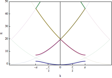
The second easy limit is when $V_0$ is very small. In particular, imagine $U=0$, Then the energies are just a parabola which is "wrapped up":


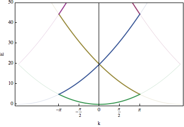
Adding finite $V_0$ at first only makes a change where bands "touch". For example, imagine $k$ is near $\pi$: $k=\pi-q$, with $q$ small. Including only the two bands which are nearly degenerate the equations are
\begin{equation}
E \left( \begin{array}{c}
u_0\\
u_1
\end{array}
\right)
= \left(
\begin{array}{cc}
(\pi-q)^2/2&U/2\\
U/2&(\pi+q)^2/2
\end{array}
\right).
\end{equation}
The eigenvalues are $E=\frac{\pi^2+q^2}{2}\pm \sqrt{(\pi q)^2+U^2/4}$, and the crossing becomes an "avoided crossing." Here is an example of numerically solving for the entire bandstructure: