To understand atoms heavier than Hydrogen, we need to know how to describe quantum mechanical systems of more than one particle. We did a bit of this when talking about Bell's inequalities, but here we will look at things more systematically. We will also encounter the concept of
``quantum statistics."

Two Particle Wavefunctions

Suppose I have two particles: a proton and an electron. Previously we assumed that the proton was ``nailed down." In principle, however, it can move, and we should use quantum mechanics to describe it. The most obvious generalization of our rules of single-particle quantum mechanics is to introduce a wavefunction, which is a function of two variables, $\psi(r_e,R_p)$. The probability density of having the electron at position $r_e$ and the proton at position $R_p$ is
\begin{equation}
P(r_e,R_p)= |\psi(r_e,R_p)|^2.
\end{equation}
This is known as the ``joint probability distribution."
The probability density of having the electron at $r_e$, regardless of where the proton may be, is
\begin{equation}
P(r_e) = \int d R_p\, |\psi(r_e,R_p)|^2.
\end{equation}
The most obvious generalization of the time-dependent Schrodinger equation is
\begin{equation}
i\partial \psi(r_e,R_p)= -\frac{\nabla_e^2}{2m_e} \psi(r_e,R_p)- \frac{\nabla_p^2}{2M_p} \psi(r_e,R_p)+V(r_e,R_p),
\end{equation}
where $V(r_e,R_p)$ is the potential energy of the system. For example, to model Hydrogen one would use
\begin{equation}
V(r_e,R_p)= -\frac{e^2}{4\pi\epsilon_0}\frac{1}{|r_e-R_p|}.
\end{equation}
In your homework you will see how to transform coordinates to reduce this to a one-particle equation.

Exchange Statistics

The last section was pretty mechanical. In this section, however, we will touch on the profound.
According to quantum mechanics electrons are indistinguishable: Suppose I have an electron in my left hand, and another in my right. I put the left electron on the table, and the right electron on the floor. I claim that state is {\em the same} as the one where I put the right electron on the table and the left on the floor. This is a highly quantum mechanical phenomenon. It means that when you start counting the states in your Hilbert space, there are a lot fewer states than you would expect. We will do some of the precise counting in two weeks. For now it suffices to grasp that classically there are two state corresponding to an electron on the floor and an electron on the table -- even if they had identical properties. I am claiming there is just one state.

If you accept this premise, then it has profound consequences. Imagine I have two identical particles (say electrons), and I move them around to "exchange" their positions

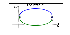
According to our axiom, there is only one state with the particles at those positions -- so I haven't done anything to the wavefunction. This is not quite true -- I might have picked up a phase factor $e^{i \phi}$.

I now imagine doing the same exchange again. If I draw the total path, I have just moved each particle around in a circle:

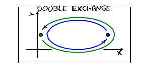
The total phase gained is obviously $e^{2i\phi}$.

The proof involves asking what happens when you continuously deform paths.
When we talk about magnetic fields we will find that you can relate the total phase picked up by a particle moving in a closed path to the flux enclosed. Thus, in the absence of a magnetic field, the phase should not depend upon the path.
Both of the loops that the particles undergo can be continuously deformed into points. We can then conclude that (in the absence of a magnetic field) the phase factor must be $1$: ie $e^{2i\phi}=1$. There are then two choices $\phi=0,\pi$. It turns out that in nature we see both types of particles: the former are said to obey ``Bose-Einstein" statistics, while the latter obey ``Fermi-Dirac" statistics.

dimensionality

The argument in the last section required that I could shrink the paths to points. It turns out that we have trouble if during that process the two particles ever touch.
The issue is that if they come together and then separate, I loose the notion of which particle is which. IE.There is no way to tell the difference between the following two trajectories:

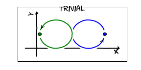
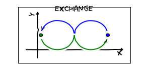
In such a case there is no constraint on $\phi$.

In three or higher dimensions it is always possible to shrink the loops in such a way that the particles never touch. Thus in those dimensions the only possible statistics are Bose-Einstein or Fermi-Dirac.
In two dimensions more complicated ``anyon" statistics are allowed. [The most famous example is the fractional quantum Hall effect.]
In one dimension I am not even sure how to define an exchange -- since any attempt to switch the positions of particles will inevitably put them in contact.
You may hear the terms "bosonization" and "fermionization." These are mathematical tricks which take advantage of this ambiguity in 1D.

wavefunction symmetry

The exchange statistics puts a constraint on the wavefunction. If $\psi(r_1,r_2)$ represents the amplitude of having particles at positions $x_1$ and $x_2$. If I reverse the ordering, I have exchanged them. Thus
\begin{equation}
\psi(r_1,r_2)=\pm \psi(r_2,r_1).
\end{equation}
The $+$ sign corresponds to bosons, and the $-$ to fermions. More generally, for an $n$-body wavefunction,
\begin{equation}
\psi(r_1,\cdots,r_i,\cdots,r_j,\cdots)=\pm \psi(r_1,\cdots,r_j,\cdots,r_i,\cdots).
\end{equation}

ground state of non-interacting particles

In the absence of interactions, The two-body wavefunction satisfies
\begin{equation}\label{2bsq}
(H_1+H_2)\psi(r_1,r_2)=E \psi(r_1,r_2),
\end{equation}
where
\begin{equation}
H_j=\frac{p_j^2}{2m}+V(r_j),
\end{equation}
with $p_j=-i\nabla_j$.
Both bosons and fermions obey the same Schrodinger equation, they just have different boundary conditions under exchange. We should be able to build the
solutions to Eq.~(\ref{2bsq}) from the single particle eigenstates:
\begin{equation}
H_1 \phi_n(r_1)=\epsilon_n \phi_n(r_1),
\end{equation}
where $n=1,2,\cdots$ labels the energies from lowest to highest.
After a little fiddling, one realizes that the following states are eigenstates of the two-body Schrodinger equation
\begin{equation}\label{2b}
\psi(r_1,r_2)\propto \phi_n(r_1) \phi_m(r_2)\pm \phi_m(r_1) \phi_n(r_2),
\end{equation}
with energy $E=\epsilon_n+\epsilon_m$.

The lowest energy state is the one with $n=m=1$. This works for bosons, but if I take the $-$ sign, the right hand side of Eq.~(\ref{2b}) vanishes. Thus the lowest energy fermionic state is $n=1,m=2$. To
summarize, the lowest energy bosonic state is
\begin{equation}
\psi(r_1,r_2)=\phi_1(r_1)\phi_1(r_2)
\end{equation}
while the lowest energy fermionic state is
\begin{equation}
\psi(r_1,r_2)=\frac{1}{\sqrt{2}}\left[\phi_1(r_1)\phi_2(r_2)-\phi_2(r_1)\phi_1(r_2)\right].
\end{equation}
Generalizing this the $N$ particles is straightforward,
\begin{eqnarray}\label{mbv}
\psi_B(r_1,r_2,\cdots,r_N)&=&\phi_1(r_1)\phi_1(r_2)\cdots\phi_1(r_N)\\\nonumber
\psi_F(r_1,r_2,\cdots,r_N)&=&\frac{1}{\sqrt{N!}}\left[\phi_1(r_1)\phi_2(r_2)\cdots\phi_N(r_N)\right.\\\nonumber&&\qquad\qquad \left.-\phi_2(r_1)\phi_1(r_2)\cdots\phi_N(r_N)+\cdots \right]
\end{eqnarray}
where in the last line we add and subtract all $N!$ ways of putting $N$ distinct $r$'s in $N$ distinct $\phi$'s. [There are $N$ choices for the first $\phi$, $N-1$ for the second, and so on.] The
signs are chosen so that you get a minus sign whenever you exchange two particles. The mathematics of all these exchanges is quite rich -- but the bottom line is it works. The simplest way to understand it is to write down the 3-particle wavefunction (which you will do in homework).
The energies of these two states are $E_B=N \epsilon_1$, and $E_F=\epsilon_1+\epsilon_2+\cdots\epsilon_N$.

Although it probably will not matter to you, unless you go on to take a solid state physics class,
we have a shorthand for the fermionic wavefunction. We note that it is equal to a determinant.
[If you don't remember what a determinant is, you can take this to be the definition.]
\begin{equation}
\psi_F(r_1,r_2,\cdots,r_N)=\frac{1}{\sqrt{N!}}\left|
\begin{array}{cccc}
\phi_1(r_1)&\phi_2(r_1)&\cdots&\phi_N(r_1)\\
\phi_1(r_2)&\phi_2(r_2)&\cdots&\phi_N(r_2)\\
\vdots\\
\phi_1(r_N)&\phi_2(r_N)&\cdots&\phi_N(r_N)
\end{array}
\right|.
\end{equation}
This is often known as a ``Slater Determinant". The fermionic symmetry is embedded in the fact that the sign of a determinant flips if two rows or columns are exchanged.

Hartree-Fock

Not only are Eqs.~(\ref{mbv}) the exact solution to the non-interacting many-body problem of a system of identical particles. They also act as a great ansatz for variational calculation of interacting particles. Typically one lets the functions $\phi_j$ be variational parameters, then minimize the energy. This is known as the Hartree-Fock approximation.
The Hartree Fock approach has been so successful that now its used as a benchmark for anything else one does. Its modern incarnation is ``density functional theory" (DFT).
A problem for which Hartree-Fock (or DFT) does poorly is known as ``strongly correlated".

physical examples

Electrons are fermions. Protons are fermions. Neutrons are fermions. Does nature only admit fermions?

No. First, there are composite bosons, such as hydrogen. Hydrogen has one proton and one electron. If you exchange it with another hydrogen atom, you get two minus signs: one from the electrons, and one from the protons. These minus signs cancel, and you effectively get a boson. Any particle made up of an even number of fermions is a boson, any made up of an odd number of fermions is a fermion.

This has cool results. Take, for example, Lithium. There are two stable isotopes of lithium $^{6}$Li and $^{7}$Li, which only differ by their number of neutrons. If you trap bosonic lithium in a harmonic potential and cool it to nK temperatures, you will find all of the atoms are in the harmonic oscillator ground state. This is a "Bose-Einstein condensate". On the other hand, if you trap fermionic lithium in the same potential, it will occupy the first $N$ level os the oscillator. You just look at the clouds, and they are of different sizes.

Nature also has a few fundamental bosons: photons, $W,Z^\pm$, gluons, and the Higgs. Having said that, there is nothing wrong with being a composite particles. Protons and neutrons are composites (like all other baryons they are made up of 3 quarks each -- quarks are fermions). If you take two quarks you can make a meson (such as a pion) which will then be a boson.

Spin-Statistics Theorem

Spin and statistics are all related to symmetries. It turns out that if you assume Lorentz invariance, you find that there are some constraints on the spins of identical particles. All relativistic bosons have spins which are a multiple of an integer, while all relativistic fermions have spins which are odd multiples of a half integer.
For example, photons and pions are bosons -- they have spin 1 and 0, and electrons and protons are fermions, and they have spin 1/2. Unfortunately I am unaware of any {\em elementary} derivation of this connection.