Last day we began discussing multi-electron atoms, and used the variational principle to derive the "Hartree" approximation. The Hartree approximation, can also be motivated on pure physical grounds. The idea is that each electron feels a potential which is the combination of the force from the nucleus, and the force from all the other electrons. Thus it obeys a Schrodinger equation
\begin{equation}
E_j \phi_j(r)= \left(-\frac{\hbar^2}{2m} \nabla^2+ V_{\rm eff}(r)\right)\phi_j(r),
\end{equation}
where
\begin{equation}
V_{\rm eff}(r) =\frac{Z e^2}{4\pi\epsilon_0} \frac{1}{|r|} +\int dr^\prime\, \frac{ e^2}{4\pi\epsilon_0} \frac{1}{|r-r^\prime|} \rho(r^\prime).
\end{equation}
Actually, for an atom it is probably slightly better to use
\begin{equation}
V_{\rm eff}(r) =\frac{Z e^2}{4\pi\epsilon_0} \frac{1}{|r|} +\left(1-\frac{1}{N}\right)\int dr^\prime\, \frac{ e^2}{4\pi\epsilon_0} \frac{1}{|r-r^\prime|} \rho(r^\prime),
\end{equation}
as there are only $N-1$ electrons that each electron sees.
This $V_{\rm eff}$ looks daunting, but its qualitative behavior is clear. If we are far away from the nucleus, then we imagine all of the charge is at a point, and and we will see something like the coulomb potential of a point particle with charge $e$. This is referred to as ``screening". If we are very close, we see the bare nucleus, and hence a potential from a point particle with charge $Z e$. The resulting potential should look something like this:
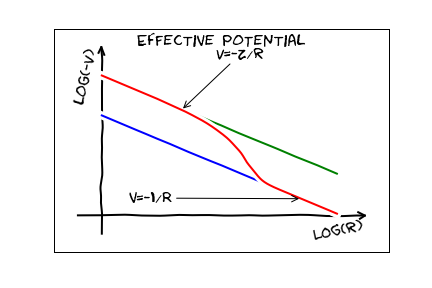
The eigenstates here will look pretty similar to the hydrogen eigenstates, but since this has fewer symmetries, the energy will depend on both $n$ and $\ell$.
Wavefunctions of particles with spin
Lets consider a single spin-1/2 particle in one dimension. It can be described by a wavefunction which takes as its arguments both the position, and the spin-projection along the $\hat z$ axis,
\begin{equation}
\psi(x,\sigma).
\end{equation}
Here $x$ is a real number, and $\sigma$ is either $1/2$ or $-1/2$ -- or more pictorially $\uparrow,\downarrow$. Sometimes it is convenient to write this as a vector
\begin{equation}
\vec\psi(x)= \left(\begin{array}{c} \psi(x,\uparrow)\\ \psi(x,\downarrow)\end{array}\right).
\end{equation}
Yet another notation is to write
\begin{equation}
\psi(x,\sigma)= \psi(x,\uparrow) \delta_{\sigma,\uparrow}+ \psi(x,\uparrow) \delta_{\sigma,\downarrow}.
\end{equation}
Different authors will choose different notation for the Kroniker delta's. For example, a reasonable, but not universal, notation is to write
\begin{equation}
\uparrow_\sigma=\delta_{\sigma,\uparrow}.
\end{equation}
Some authors even just let the $\sigma$ be implicit. I do not recommend leaving it out until you become an expert.
A two-electron wavefunction in one-dimension would have the form
\begin{equation}
\psi(x_1,x_2,\sigma_1,\sigma_2).
\end{equation}
Just as the one-electron wavefunction could be thought of as two functions, this one can be thought of as four functions,
\begin{eqnarray}
\psi(x_1,x_2,\uparrow,\uparrow)\\
\psi(x_1,x_2,\uparrow,\downarrow)\\
\psi(x_1,x_2,\downarrow,\uparrow)\\
\psi(x_1,x_2,\downarrow,\downarrow).
\end{eqnarray}
Fermionic symmetry requires that
\begin{equation}
\psi(x_1,x_2,\sigma_1,\sigma_2)=-\psi(x_2,x_1,\sigma_2,\sigma_1).
\end{equation}
This is often (but not always) achieved by separately symmetrizing/antisymmetrizing the spatial and spin parts of the wavefunction. For example
\begin{eqnarray}\label{sym}
\psi(x_1,x_2,\sigma_1,\sigma_2)&=& f(x_1,x_2) \left(\uparrow_{\sigma_1} \downarrow_{\sigma_2}-\downarrow_{\sigma_1} \uparrow_{\sigma_2}\right)\\
f(x_1,x_2)&=& f(x_2,x_1).
\end{eqnarray}
Another common structure you see is
\begin{eqnarray}\label{anti}
\psi(x_1,x_2,\sigma_1,\sigma_2)&=& f(x_1,x_2) \uparrow_{\sigma_1} \uparrow_{\sigma_2}\\
f(x_1,x_2)&=&-f(x_2,x_1).
\end{eqnarray}
Hund's rule is mainly the statement that typically the electron-electron interaction energy is less in wavefunctions of the form of Eq.~(\ref{anti}) than that of (\ref{sym}). This kind of makes sense since there must be a node in $f$ for the antisymmetric spatial wavefunction.
Helium
At this point, I am itching to do a real calculation. Lets see if we can estimate the binding energy of Helium. If we wanted to do the problem right, we would solve the following six-dimensional partial differential equation,
\begin{equation}\label{big}
E\psi(r_1,r_2,\sigma_1,\sigma_2) =\left[-\frac{\hbar^2\nabla_1^2}{2 m} -\frac{\hbar^2\nabla_2^2}{2 m} -\frac{2 e^2}{4\pi\epsilon_0} \left(\frac{1}{r_1}+\frac{1}{r_2}\right) + \frac{e^2}{4\pi \epsilon_0} \frac{1}{|r_1-r_2|}\right]
\psi(r_1,r_2,\sigma_1,\sigma_2)
\end{equation}
with the condition
\begin{equation}
\psi(r_1,r_2,\sigma_1,\sigma_2)=-\psi(r_2,r_1,\sigma_2,\sigma_1).
\end{equation}
Makes my brain hurt.
Since spin does not explicitly appear in the differential equation (just the boundary condition), we can always find solutions of one the form in Eq.~(\ref{anti}) or (\ref{sym}). Note that this ignores a relativistic effect known as "spin-orbit coupling" which gives the splitting of the d-lines in sodium. The spin-antisymmetric wavefunctions are known as "Para" helium. The spin symmetric ones are "ortho" helium. We want the ground state, which will be Para, as that lets us put both electrons in an s-state.
The first thing we do with a problem like this is dimensional analysis. There is only one quantity here with the dimension of energy
\begin{equation}
E_0=-13.6eV.
\end{equation}
Thus we know $E= {\cal E} E_0$, where $\cal E$ is some number which should not be so different from 1. Experiments find that $E=-78.9754eV=5.8 E_0$. Our goal is to come up with that $5.8$.
Adimensionalizing Eq.~(\ref{big}) with the Bohr radius and the Rydberg yields
\begin{equation}
{\cal E} \psi = \left[-\frac{\nabla_1^2}{2 } -\frac{\nabla_2^2}{2 } -\frac{2}{r_1}-\frac{2}{r_2} + \frac{1}{|r_1-r_2|}\right]\psi.
\end{equation}
Our next step is to throw away the electron-electron interaction. Is that a good approximation? No. But it gives us a problem we can solve. We will then estimate the size of the electron-electron interaction energy. Without the coupling term, the equation is separable, and we can write the wavefunction as a product
\begin{equation}
\psi(r_1,r_2)=\phi_1(r_1)\phi_2(r_2).
\end{equation}
We should then symmetrize this wavefunction, but lets first not worry about that. In fact, we expect $\phi_1=\phi_2$, so this is already symmetrized. Plugging this ansatz into the Schrodinger equation yields
\begin{equation}
{\cal E} = {\cal E}_1+{\cal E}_2
\end{equation}
with
\begin{equation}
{\cal E}_1 \phi_1 = -\frac{\nabla_1^2}{2 } \phi_1 - \frac{2}{|r_1|} \phi_1,
\end{equation}
and the same for $\phi_2$.
We can use scaling to solve this equation. We know that if we did not have that $2$ there, the lowest energy solution would have $\cal E=-1$. We can write it in that form by making the transformation $r_1=\lambda s$, which yields
\begin{equation}
{\cal E}_1 \phi_1 = -\frac{\nabla_s^2}{2 \lambda^2 } \phi_1 - \frac{2}{\lambda |s|} \phi_1,
\end{equation}
or equivalently
\begin{equation}
\lambda^2 {\cal E}_1 \phi_1 =-\frac{\nabla_s^2}{2} \phi_1 - \frac{2 \lambda}{|s|} \phi_1.
\end{equation}
If I take $\lambda=1/2$, I get exactly the equation for hydrogen. Thus $(1/4) {\cal E}_1=-1$. By symmetry the same can be said for ${\cal E}_2$. Thus, if we neglect electron-electron interaction we get
\begin{equation}
{\cal E}= -8.
\end{equation}
Now a crude estimate of the electron-electron interaction is that it should be something like
\begin{equation}
{\cal E}_{ee}= \langle \frac{1}{|r_1-r_2|} \rangle.
\end{equation}
If we take $\langle 1/|r_1-r_2|\rangle\approx\lambda$, this gives ${\cal E}_{ee}\sim2$, and ${\cal E}=-6$, which is pretty close to the experimental value of ${\cal E}=-5.8$. The agreement is actually even better -- next week we will actually calculate the average, and find ${\cal E}_{ee}=5/(4\lambda)=5/2$, which gives ${\cal E}\approx-5.5$, which is really close. We will also use the variational method to get ${\cal E}\approx -5.7$, which is good enough for me.