The number one skill we are trying to develop in this course is Modeling. That is we want to be able to take a physical situation, and put a mathematical framework around it. In most of your courses, the models have been presented to you, and your task was to figure out how to correctly apply a given model. Now we want you to develop models. This is a hard task, so the first few times, I am going to walk you through it.
Our first few examples will involve dynamics. Dynamics problems are nice because they are concrete. You start the system in some known configuration, then ask how it evolves. By understanding these physical problems, you will get intuition about aspects of quantum mechanics which can feel a bit abstract..
One thing to point out is that this is only our second lecture. Thus part of my goal is to get all of us on one notational footing. Some of today's discussion is meant to feel familiar, and give you new notation for things you already know. I hope that afterwards you will have deeper insight into the physical meaning of wavefunctions.
Measuring wavefunctions
The system we will model today is a ``Bose-Einstein Condensate" of Rubidium atoms. These are atoms which are trapped in a magnetic bottle, and cooled to the quantum ground state. Since each Rubidium atom is identical, they are all in the same single-particle state. That is the wavefunction $\psi(r)$ for one atom is the same as the wavefunction for any other atom. A typical gas might have $N=10^6$ atoms, and be 10's of microns across. A nice concrete model for the wavefunction is a Gaussian $\psi(r)\sim \exp(-r^2/2d^2)$. Our first modeling task is to understand what the experimentalists will see if they take a photograph of their cloud. We know that if we had a single particle we would see just a single spot on the camera, and the probability of that spot being at position $r$ is proportional to $|\psi(r)|^2$. We want to model what will be seen in the limit of a large number of particles. In that limit we expect to see a blurry blob, made up of all of the individual spots. In fact the spots should be so close together that they look like a continuous density distribution. Our question is what is that density distribution. I'll repeat this again a little more clearly.
The first step to modeling is simplifying.
The experiments are in 3D space, but if we first understand the 1D case, extending it to 3D should hopefully be easy. Thus we imagine that each particle lives on a line.
If I look at where the atoms are, I will find each atom somewhere: the probability of finding particle 1 within $dx$ of position $x$ is $|\psi(x)|^2 dx.$ The probability of finding particle 2 within $dx$ of $x^\prime$ is $|\psi(x^\prime)|^2$. These are independent (or uncorrelated or unentangled), meaning that if I am generating a typical result of a measurement, I would randomly choose where particle 1 is, and separately choose where particle 2 is: the outcome of one roll of the dice does not change the other. The same thing applies to 2D or 3D. I wrote a small computer program to generate such random positions in 2D. Here are three examples with 1000 particles:
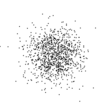
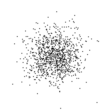
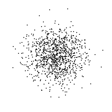
These are clearly different (the dots are in different places) but also the same (the density of dots is the same).
Now in an actual experiment, one uses a pixelized detector with finite resolution. It counts how many particles land on each pixel. This is more easily illustrated in 1D. Here is a typical 1D distribution of particles:
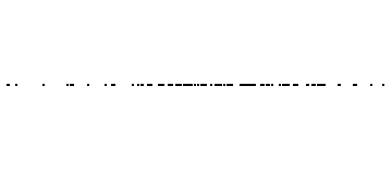
And here is the pixelized version -- for several different particle numbers:
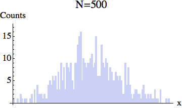
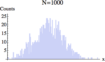
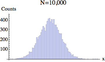
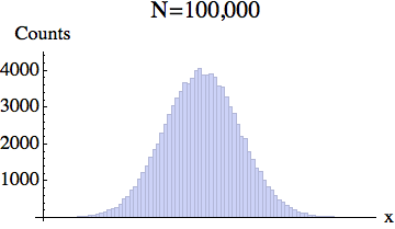
What the experiment really measures is this coarse-grained density, rather than the exact location of each particle.
We know the probability of any given particle being in a bin at position $x$ of width $dx$ is $|\psi(x)|^2 dx$. Thus the average number of particles in that bin is $\rho(x) dx=N |\psi(x)|^2 dx$. The experiment measures $\rho(x)$, and hence tells us what $|\psi(x)|^2$ is. Here is an experiment where you can explicitly measure the wavefunction (or at least the magnitude of the wavefunction)!!! I repeat, despite what you may have heard, there are cases where the wavefunction can be measured.
The generalization to 2D is obvious. The number of particles in a bin at position $x,y$ of size $dx\,dy$ is $|\psi(x,y)|^2\,dx\,dy$. It also generalizes to 3D: the number of particles in a bin at position $x,y,z$ of size $dx\,dy\,dz$ is $|\psi(x,y,z)|^2\,dx\,dy\,dz$. Unfortunately, there is one subtlety in 3D -- taking a picture does not give you 3D information. What you actually get is the "column density" -- that is the integrated density along the line of site
\begin{equation}
n_c(x,y)= \int |\psi(x,y,z)|^2 dz.
\end{equation}
Luckily, experimentalists can trap the atoms in 2D pancake traps, where this subtlety is unneccessary.
This was a simple case of modeling, but I want to reiterate what we did. First, we simplified -- went to 1D. Then we simplified some more -- asked what happens with one particle. Then we extrapolated. The lesson here is less about experiments on cold atoms, and more about modeling.
Time-of-flight
The simplest experiment one can do with this system is to simply turn off the trap. Quantum-mechanically one would model the subsequent dynamics by solving the time dependent Schrodinger equation
\begin{equation}
i\hbar\partial_t \psi(x,t)=-\frac{\hbar^2 \partial_x^2}{2 m} \psi(x,t)
\end{equation}
with initial conditions $\psi(x,0)=A e^{-x^2/2d^2}$, where $A=1/(\pi d^2)^{1/4}$ is a normalization constant. Since we measure $\psi(x,t)$, knowing how the wavefunction evolves tells us everything we need to know.
You may have solved this problem exactly in PHYS 3316, and it is fairly straightforward. In the spirit of this course, however, we are not going to focus too much on the exact solution. Instead we are going to try to understand the behavior using simple arguments. For example, today we will hone our intuition by thinking about these dynamics from a classical point of view. On tuesday of next week I will show you a powerful technique for calculating how the cloud behaves, which is simpler than what you did in PHYS 3316. You learn less, but it is easier. One of the big lessons of this course will be how to be lazy. I want to emphasize that we are not doing anything which is not already contained in the Schrodinger equation, we are just finding smart ways to understand it.
Before proceeding, I will just quote the exact result. If don't know how to get this, don't worry, I will show you how to derive this another day.
Regardless, the result is
\begin{equation}
\psi(r,t)= A(t) e^{- x^2/2 (d^2+i \hbar t/m)},
\end{equation}
where again $A(t)$ is a normalization, which depends on time.
Complete Classical Expansion worksheet.
My classical picture for what happens is that I have a bunch of atoms localized to a small region with a distribution of momenta. Let $n_p dp$ be the number of atoms with momentum within $dp$ of $p$. When I turn off the trap they all fly off. After a time $t$, the number of particles within $dx$ of position $x$ is
\begin{equation}
\rho(x,t)dx=n_{p=m x/t} \frac{m}{t} dx.
\end{equation}
Classically, the density of particles in real space after time $t$ is related to the density in momentum space at time $0$. This is also true quantum mechanically. In fact one of the lessons here is that your classical intuition is almost always right -- even in quantum mechanics.
Never abandon your classical intuition. Whenever you are stuck, ask yourself -- if this was a Physics 1112 problem, what would happen?
There are a few comments that are worth making. First, our classical analysis assumed all of the particles were at the same location. We could add some distribution of the starting locations as well. It wouldn't be too hard, but at long times it will make no difference. Second, we did not say how to get $n_p$. For that we need to turn back to quantum mechanics. As with the real-space density distribution, one expects that $n_p =N P_p$, where $N$ is the total number of atoms, and $P_p$ is the probability that a given atom has momentum $p$. According to the measurement hypothesis, the probability of measuring a particle with momentum $p$ is
\begin{eqnarray}
P_p &\propto& \left|\int\!dx\, \phi_p(x)^* \psi(x)\right|^2\\
&\propto&\left|\int\!dx\, e^{-i p x/\hbar} \psi(x)\right|^2. \label{result}
\end{eqnarray}
We again have a little subtlety about this is a continuous distribution, and what we really are defining is the probability that the particle has momemtum within $dp$ of $p$. If we require
\begin{equation}
\int dp P_p =1,
\end{equation}
then we find that the proportionality constant in Eq. (\ref{result}) is $1/2\pi$. This can also be written as
\begin{equation}
P_p=\frac{1}{2\pi} |\psi_{k=p/\hbar}|^2,
\end{equation}
where $\psi_k$ is the Fourier transform of $\psi(r)$.
Most of the time I will leave out the $\hbar$'s.   One often describes $\psi_k$ as the ``momentum space wavefunction".
From our classical argument, we should be able to measure $|\psi_k|^2$ with a time of flight experiment.
If we take the exact result and make the time large (so that the initial spread of the starting positions can be ignored) we find
\begin{eqnarray}
\psi(r,t)&=&A(t) e^{- x^2/2 (d^2+i \hbar t/m)},\\
&\to& A(t) \exp\left[ \frac{ i m x^2}{2\hbar t}\left(1+ \frac{i d^2 m}{i\hbar t}+\cdots \right)\right].
\end{eqnarray}
Thus the density is
\begin{equation}
\rho(r,t)=N|\psi(r,t)|^2 \to |A(t)|^2 \exp\left(- \frac{m^2 x^2 d^2}{\hbar^2 t^2}\right) \qquad \mbox{ for $t$ large}.
\end{equation}
We can compare that expression to the momentum space wavefunction,
\begin{eqnarray}
\psi_k&=& \int dr\, e^{i k\cdot r} A e^{- r^2/2 d^2}\\
&\propto& \exp(- d^2 k^2/2).
\end{eqnarray}
We indeed see the classical result that for long time
\begin{equation}
\rho(r,t)\propto |\psi_{k=m r/\hbar t}|^2.
\end{equation}
Note that I have used the physicist convention of using the same symbol $\psi$ for both the real and imaginary space wavefunction. This can be confusing. I at least gave you a subtle typographic clue: I used a subscript for the argument of the momentum-space wavefunction, and parentheses for the real-space wavefunction. Many authors don't even do that. When you are reading the literature you may find that you need to determine what function you are looking at by the argument. Traditionally $r,x,y,z,s$ are arguments of real-space wavefunctions, and $k,p,q$ are arguments of momentum-space wavefunctions. Thus you might see a notation like $\psi(k=m r/\hbar t)$, which means the momentum space wavefunction.
Those of you who take PHYS 4443 will see a more abstract way of thinking about different representations of wavefunctions. The real-space and momentum-space wavefunctions are just two particular cases.
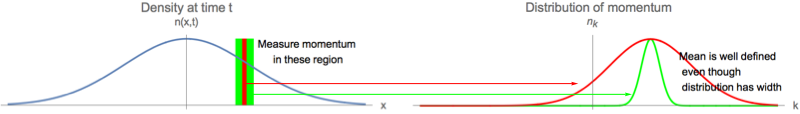
Correlation between position and momentum
The classical argument also gives an interesting observation. Classically, all of the particles at position $x$ at time $t$ have momentum $p=mx/t$. This is because only the particles moving with velocity $x/t$ would be at that location. The position and momentum are correlated for the classical distribution of particles. The same must be true of the quantum mechanical wavefunction. What does this mean when you cannot simultaneously specify the momentum and position? The solution is that if you look at a range of positions of width $\delta x$, there are a range of momenta of width $\delta p$, and the uncertainty $\delta p$ grows when you make $\delta x$ smaller. Despite the breadth of the distribution, the average momentum in that region has some definite value, which is essentially independent of the region size: