Today we extend our understanding of the modeling from last day. There we argued that measuring the density of an atomic gas gives us direct access to the square amplitude of the real-space wavefunction. We also argued that a time-of-flight experiment gives access to the square amplitude of the momentum-space wavefunction. Finally I tried to convince you that time-of-flight correlates the momentum and position of the particles. I thought that was pretty neat, but the first step in our analysis involved calculating a time dependent wavefunction. Finding the wavefunction requires solving a partial differential equation. That sounds like hard work to me, and I am intrinsically lazy. In this lecture I will show you a couple tricks which make things easier.
Correlation between position and momentum
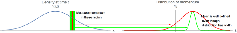
The classical argument also gives an interesting observation. Classically, all of the particles at position $x$ at time $t$ have momentum $p=mx/t$. This is because only the particles moving with velocity $x/t$ would be at that location. The position and momentum are correlated for the classical distribution of particles. The same must be true of the quantum mechanical wavefunction. What does this mean when you cannot simultaneously specify the momentum and position? The solution is that if you look at a range of positions of width $\delta x$, there are a range of momenta of width $\delta p$, and the uncertainty $\delta p$ grows when you make $\delta x$ smaller. Despite the breadth of the distribution, the average momentum in that region has some definite value, which is essentially independent of the region size:
Work through the Continuity handout.
A useful framework for understanding this local velocity, is to write the complex wavefunction as an amplitude and a phase
\begin{equation}
\psi(x,t)= f(x,t) e^{i\phi(x,t)},
\end{equation}
where both $f$ and $\phi$ are real. The Schrodinger equation reads
\begin{eqnarray}
i\partial_t \psi(x,t) &=& -\frac{1}{2m} \partial_x^2 \psi(x,t)\\
i \partial_t f(x,t) e^{i \phi(x,t)} &=& -\frac{1}{2m} \partial_x^2 f(x,t) e^{i\phi(x,t)}
\end{eqnarray}
We now apply the chain rule to simplify this. The trickiest part is the second derivative with respect to $x$. I like to do this in steps
\begin{equation}
\partial_x \left[ f e^{i \phi} \right] =( \partial_x f) e^{i \phi} + i (f\partial_x \phi) e^{i \phi}.
\end{equation}
We then apply a second derivative
\begin{eqnarray}
\partial_x^2 \left[ f e^{i \phi} \right] &=& \partial_x \left[
( \partial_x f) e^{i \phi} + i (f\partial_x \phi) e^{i \phi}
\right]\\
&=&
\left(\partial_x^2 f - f (\partial_x \phi)^2 + 2 i \partial_x f \partial_x\phi+i f \partial_x^2 \phi \right) e^{i\phi}.
\end{eqnarray}
This brings us to
\begin{eqnarray}
i(\partial_t f) e^{i \phi} -(f \partial_t \phi) e^{i\phi} &=&
-\frac{1}{2m}\left(\partial_x^2 f - f (\partial_x \phi)^2 \right)e^{i\phi}
\\ \nonumber&&
-\frac{i}{2m}\left(
2 \partial_x f \partial_x\phi + f \partial_x^2\phi\right) e^{i\phi}
\end{eqnarray}
We then multiply by $e^{-i\phi}$ and take the real and imaginary parts. Both are interesting, but for our purposes, we will get the most out of the imaginary part, which is
\begin{eqnarray}
\partial_t f +\frac{1}{2m} \left[2 \partial_x f \partial_x \phi + f \partial_x^2\phi\right] &=&0.
\end{eqnarray}
The canonical way to write this is to multiply by $2f$, and note
\begin{equation}
2 f\partial_t f = \partial_t f^2 = \partial_t n,
\end{equation}
where $n$ is the density. Thus
\begin{eqnarray}
\partial_t n + \frac{1}{m} \left[\partial_x n \partial_x \phi + n \partial_x^2 \phi \right]&=&0\\
\partial_t n + \partial_x \left[ n \frac{\partial_x \phi}{m}\right] &=&0.
\end{eqnarray}
The form of equation is very common in physics. You see it in fluid mechanics, electromagnetism... It is known as the continuity equation, and is typically written as
\begin{equation}
\partial_t n + \partial_x j =0.
\end{equation}
If we went through the same argument in 3D we would have found
\begin{equation}
\partial_t n + \nabla\cdot {\bf \vec j} =0,
\end{equation}
where the particle current is
\begin{equation}
\nabla\cdot \vec {\bf j} = \frac{n(r,t)}{m} \nabla \phi(r,t).
\end{equation}
The physics of the continuity equation is that the rate of change of the local density is given by the difference between the flow into some volume and the flow out. Mathematically the differences between flows is given by the divergence. The current can be thought of as a density times an average velocity. Thus we see that the average velocity at location $\bf r$ is
\begin{equation}
{\bf v}({\bf r},t) = \frac{1}{m} \nabla \phi({\bf r},t),
\end{equation}
which gives us physical meaning to the phase of the wavefunction. If you want to use physical units (where $\hbar\neq 1$), you can use dimensional analysis to write
\begin{equation}
{\bf v}({\bf r},t) = \frac{\hbar}{m}{ \nabla \phi({\bf r},t)}.
\end{equation}
We will talk more about dimensional analysis in the future, and you will become more comfortable with this glibness with $\hbar$'s.
It turns out that you have seen this local current before in PHYS 3316. You may remember discussing "probability current," defined by
\begin{equation}
{\bf j} = \frac{\hbar}{2 m i} \left[\psi^*\nabla \psi - \psi \nabla \psi^*\right].
\end{equation}
I will leave it as an exercise to show that this is the same as the $\bf j$ that we defined in terms of the phase of the wavefunction.
Regardless, we can now take our solution to the time dependent Schrodinger equation
\begin{equation}
\psi(x,t)\approx A(t) \exp\left[ \frac{ i m x^2}{2\hbar t}\left(1+ \frac{i d^2 m}{i\hbar t}+\cdots \right)\right].
\end{equation}
What is $v(x,t)$? How does it compare with the classical prediction?
Heisenberg's equations of motion
The first trick is to only calculate what you really want to know. Lets think about this. I am doing an experiment. I have a bunch of atoms trapped in a tight trap. I turn off the trap and it expands. I have the ability to take pictures of the cloud as it expands. I want to model the experiment, and prove to my colleagues that I understand what is going on.
Last day we argued that one way to model the experiment was to solve the time-dependent Schrodinger equation. The density I measure is exactly $|\psi|^2$. I could then make a bunch of plots which show the measured density, and $|\psi|^2$, and see if they agree. Suppose it is a two-dimensional experiment. I then have a three-dimensional data set (because I have time). How am I going to plot this? How am I going to organize this data?
One approach is to extract one number from each density profile which characterizes it. The natural thing to look at is the size of the cloud. There are many ways to characterize the size, but from experience I know that the easiest one to calculate will be the root-mean-square width:
\begin{equation}
\sigma(t)=\langle x^2\rangle = \int\, dx\, x^2\, |\psi(x,t)|^2.
\end{equation}
Here we will try to calculate equations of motion for this quantity without calculating the wavefunction. I believe this trick was invented by Dirac when he reconciled Heisenberg's matrix mechanics and Schrodinger's wave mechanics (though Schrodinger may have came up with it first). The idea is to simply take the derivative of $\sigma(t)$
\begin{equation}
\partial_t \sigma(t) = \partial_t \int dx\, x^2\, |\psi(x,t)|^2.
\end{equation}
We then use the linearity of the integral to take the derivative inside
\begin{equation}
\partial_t \sigma(t) = \int dx\, x^2\, \left[\psi^*\partial_t \psi +(\partial_t \psi^*) \psi\right].
\end{equation}
We now use the Schrodinger equation,
\begin{equation}
i\partial_t \psi = H \psi
\end{equation}
and its conjugate
\begin{equation}
-i \partial_t \psi^* = (H \psi)^*
\end{equation}
to write
\begin{equation}
\partial_t \sigma(t) = \int dr\, r^2\, \frac{1}{i}\left[\psi^*H \psi -(H \psi)^* \psi\right].
\end{equation}
Note, that I am being a little obtuse by writing $(H\psi)^*$ instead of $(H \psi^*)$. The reason is that for an arbitrary operator, these things are in fact different.
In the case at hand
\begin{equation}
H=-\frac{1}{2m} \partial_x^2
\end{equation}
this distinction is meaningless, and we have
\begin{equation}
\partial_t \sigma(t) = \frac{-1}{2m} \int dx\, x^2\, \frac{1}{i}\left[\psi^* \partial_x^2 \psi -(\partial_x^2 \psi^*) \psi\right].
\end{equation}
We then integrate the second terms by parts twice,
\begin{eqnarray}
\partial_t \sigma(t) &=& \frac{-1}{2m} \int dx\, \frac{1}{i}\left[ \psi^* \partial^2_x \psi -\psi^* \partial_x^2 (x^2 \psi)\right]\\
&=& \int dx\, \psi^* \frac{1}{i} (x^2 H - H x^2) \psi
\end{eqnarray}
where by $H x^2 \psi$ I mean $H (x^2\psi)$. Following this logic, one writes
\begin{equation}
\partial_t \langle x^2\rangle = \langle \frac{1}{i}( x^2 H - H x^2) \rangle = \frac{1}{i} \langle [x^2,H]\rangle.
\end{equation}
It is clear that we can replace $x^2$ by any reasonable linear operator, and we would get the same structure. This logic will also go through for any $H$ which obeys the property
\begin{equation}
\int dx\, (H\psi)^*(x) \phi(x) = \int dx\, \psi^*(x) (H \phi)(x),
\end{equation}
for any functions $\psi$ and $\phi$.
We call such operators Hermitian. This Hermitian property is necessary for the Schrodinger equation to make sense.
As with many physics tricks, we seem to have made things worse, rather than better. We have gained, however, the ability to use a symbolic language to answer the question of how cloud expands. For example, you are probably familiar with the statement
\begin{equation}
[x,p]=i.
\end{equation}
This is short-hand for the observation
\begin{equation}
x \frac{1}{i}\partial_x \psi(x) - \frac{1}{i}\partial_x \left( x \psi(x)\right) = i \psi(x).
\end{equation}
We can use these, and similar statements to simplify the equations of motion.
One useful identity is
\begin{eqnarray}
[A,BC]&=&ABC-BCA\\
&=&(A B-BA)C + B (AC-CA)\\
&=& [A,B] C+ B [A,C].
\end{eqnarray}
A second is
\begin{eqnarray}
[AB,C]&=& ABC-CAB\\
&=& A (BC-CB)+ (AC-CA)B\\
&=& A [B,C]+[A,C] B.
\end{eqnarray}
Combining these yields
\begin{eqnarray}
[AB,CD] &=& A [B,CD]+[A,CD]B\\
&=& A C [B,D] + A[B,C]D+C [A,D]B+[A,C]DB.
\end{eqnarray}
With these we see
\begin{eqnarray}
[x^2,p^2] &=& x p [x,p]+ x [x,p] p+ p [x,p] x + [x,p] p x\\
&=& 2i (xp+px).
\end{eqnarray}
We therefore have
\begin{equation}
\partial_t \langle x^2 \rangle = \frac{1}{i}\langle [x^2,H ]\rangle=\frac{1}{m} \langle xp+px \rangle.
\end{equation}
Note the similarity with the classical equation $\partial_t x^2 = 2 xp/m$. The only difference is in the ordering of operators.
We then take another derivative,
\begin{equation}
\partial_t \langle xp \rangle =\frac{1}{i} \langle [xp,H]\rangle = \frac{1}{2 i m } \langle [xp,p^2]\rangle.
\end{equation}
This one is even easier
\begin{eqnarray}
[xp,p^2] &=& 2 i p^2.
\end{eqnarray}
Similarly
\begin{eqnarray}
[px,p^2] &=& 2 i p^2.
\end{eqnarray}
Thus we have
\begin{equation}\label{heis1}
\partial_t^2 \langle x^2\rangle = \frac{2}{m} \langle p^2\rangle.
\end{equation}
Lets try one more derivative
\begin{equation}
\partial_t \langle p^2\rangle = \frac{1}{i} \langle [p^2,H]\rangle.
\end{equation}
In the present case, the only operator in $H$ is $p$, so $[p^2,H]=0$. Thus $\langle p^2\rangle$ does not change with time. This is nothing but the classical observation that in free expansion the momentum of the particles does not change.
We can now integrate Eq.~(\ref{heis1}), finding
\begin{equation}
\langle x^2\rangle(t) = d^2 + s_0 t + \frac{ 2 p_0^2}{m} t^2,
\end{equation}
where $d^2$ and $s_0$ are constants of integration, having to do with the initial conditions. At long times the quadratic term dominates, and the width grows linearly with time. The speed of growth tells us about the root-mean-square velocity distribution.
The remarkable thing is that our result is completely general. We did not assume a Gaussian wavepacket. In fact
we never needed to calculate the wavefunction. The cost, however, is that our theory contains a free parameter, $p_0^2 = \langle p^2 \rangle$. Is that a bad thing? No, it is a great thing. We can walk into the lab and measure $\langle x^2(t)\rangle$. If it is quadratic at long times, then we have somewhat validated our theory. We can then extract from the experiment our unknown quantity $\langle p^2\rangle$.
How good is this? Well here is some sample data from Holland, Jin, Chiofalo and Cooper, Phys. Rev. Lett. 78, 3801 (1997),
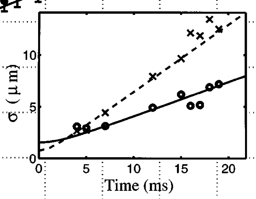
The points are data, and the lines are essentially the theory we used. The cloud in these experiments was oblong, so the two different curves correspond to the two principle axes.
Coherence
At this point you should be pretty bored. We just spent three classes finding a result which might as well be derived by classical fluid mechanics. How do I know this is really quantum mechanical? If I led you into a lab, is there anything you could do to show the failure of classical mechanics?
We didn't have time to discuss this in class, but if you are curious, here is a nice example.
One approach is instead of using a single cloud, you use two. Suppose the two clouds are initially separated by a distance $d$. Consider some point a distance $x_0$ away from one cloud (and hence a distance $d-x_0$ away from the other). By our classical argument the atoms that reach that point at time $t$ have momenta $m x_0/t$ and $m (x_0-d)/t$. Near that point we can think of them as plane waves
\begin{equation}
\psi(x) \sim A e^{i m x_0 x/t} + B e^{i m (x_0-d) x/t}.
\end{equation}
The density near that point will then be
\begin{equation}
\rho(x)=|\psi(x)|^2 = |A|^2 + |B|^2 + 2 {\rm Re} ( B^* A e^{i m d x/t}).
\end{equation}
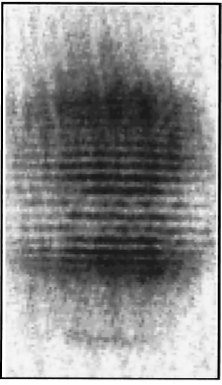
The interference term oscillates with a wavelength $\lambda= t/(m d)$. Interestingly, this wavelength is independent of $x_0$, so one expects to see evenly spaced fringes. The result of the experiment? In Science 275, 637 (1997), Andrews, Townsend, Miesner, Durfee, Kurn, and Ketterle saw images like this one
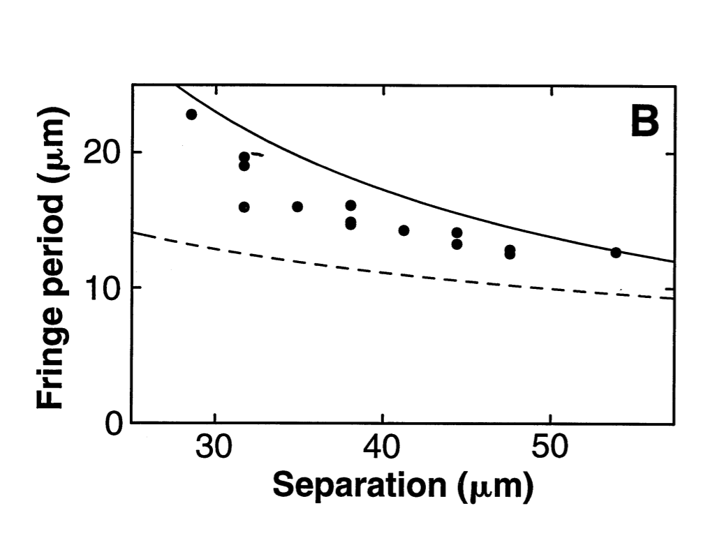
Moreover, when they looked at the fringe spacing as a function of $d$, they found excellent agreement with this simple theory (shown as the solid curve)
A few comments are in order: First, we only did extremely simple math. The most complicated thing we did here was adding two complex exponentials. Second, we combined classical and quantum reasoning. Yes, it took us two lectures to come to the understanding that you can get away with this, but once you understand the possibility, the arguments are easy.
General Wave-Packet Dynamics
I probably will not have time for this section in class, but I wanted to mention yet another way to calculate the motion of a wave-packet. This is closer to what you did in PHYS 3316. We will come back to this when we talk about solid state physics, so it is not critical to do this now.
We imagine that at time $t=0$ we have a relatively localized wave-function $\psi(x,0)$ -- maybe describing a cloud of atoms dropped from a trap. We want to solve the time-dependent Schrodinger equation
\begin{equation}
i\partial_t \psi = - \frac{1}{2m}\partial_x^2 \psi.
\end{equation}
Our strategy come right out of MATH 2930 -- we will separate variables. We note that plane waves are eigenstates of the Laplacian,
\begin{equation}
-\frac{1}{2m} \partial_x^2 e^{i kx} = \epsilon_k e^{i k x}
\end{equation}
where $\epsilon_k = k^2/2m$. We then write our wave-function as a sum over plane waves
\begin{equation}
\psi(x,t)= \sum_k c_k(t) e^{i k x},
\end{equation}
where $\sum_k$ is short-hand for $\int dk/(2\pi)$.
We plug this into the Schrodinger equation to find
\begin{equation}
\sum_k e^{i k x} i\partial_t c_k(t) = \sum_k e^{i k x} \epsilon_k c_k.
\end{equation}
This equation must be true for all $x$, so we can equate terms in the series, yielding
\begin{equation}
c_k(t) = c_k(t) e^{-i \epsilon_k t}.
\end{equation}
Using this formal expression for the wavefunction we can calculate any quantity we want. As a good example, we can look at the center of mass position:
\begin{eqnarray}
\langle x\rangle &=& \int dx\, x\psi^*(x)\psi(x)\\
&=& \int dx\, x \sum_{kq} e^{i (q-k) x} e^{i (\epsilon_k-\epsilon_q) t}c_k^* c_q\\
&=& \sum_{kq} e^{i (\epsilon_k-\epsilon_q) t}c_k^* c_q \int dx\, x e^{i (q-k) x}
\end{eqnarray}
We want to calculate this integral with minimal assumptions about the $c$'s. The best trick I know for doing this is "differentiating under the integral." For those of you who read Feynman's light biographical books, you may remember that he was rather fond of this trick. The idea is to differentiate with respect to the momenta in order to get rid of the $x$
\begin{equation}
\int dx\, x e^{i (q-k) x} = \frac{\partial_q-\partial_k}{2i} \int dx\, e^{i (q-k) x} = \frac{\partial_q-\partial_k}{2i} 2\pi \delta(q-k).
\end{equation}
This then leads to
\begin{eqnarray}
\langle x \rangle &=& \int \frac{dk}{2\pi} \int \frac{dq}{2\pi} e^{i (\epsilon_k-\epsilon_q) t}c_k^* c_q \, \frac{\partial_q-\partial_k}{2i} 2\pi \delta(q-k).
\end{eqnarray}
We integrate by parts to find
\begin{eqnarray}
\langle x \rangle &=& \int \frac{dk}{2\pi} \int \frac{dq}{2\pi} e^{i (\epsilon_k-\epsilon_q) t}c_k^* c_q \, \frac{\partial_k \epsilon_k+\partial_q \epsilon_q }{2} t 2\pi \delta(q-k)\\\nonumber&&+ \int \frac{dk}{2\pi} \int \frac{dq}{2\pi} e^{i (\epsilon_k-\epsilon_q) t} \frac{\partial_q-\partial_k}{2i} c_k^* c_q 2\pi \delta(q-k)
\end{eqnarray}
The first term is linear in time, and the second term is independent of time, allowing us to write
\begin{eqnarray}
\langle x \rangle &=& x_0 + v t
\end{eqnarray}
where
\begin{eqnarray}
x_0 &=& \langle x\rangle(t=0)\\
v &=& \int \frac{dk}{2\pi} \partial_k \epsilon_k |c_k|^2
\end{eqnarray}
If the the $c_k$'s are sharply peaked about some wave-vector $k_0$, then the expression for the velocity can be simplified. Essentially, $\partial_k \epsilon_k$ does not change much over the region where the integral is non-zero, so it can be pulled out, yielding
\begin{equation}
v= \left.\partial_k \epsilon_k\right|_{k=k_0} = \frac{k_0}{m}.
\end{equation}
A similar argument works for $\langle x^2\rangle$, but one needs to take a second order derivative with respect to the momentum, and hence finds a quadratic dependence on time.