Well before the laser, there was a maser. This was a peculiar sort of microwave amplifier based upon a quantum effect: stimulated emission. We won't discuss stimulated emission today, rather we will focus on a key ingredient in the maser: ammonia. On Tuesday we will figure out how the Maser works.

Ammonia is an interesting molecule. It consists of 3 hydrogens, and one nitrogen, which form a pyramid. Imagine holding the hydrogens rigid, forming a triangle in the x-y plane. Now imagine moving the nitrogen atom along the z-axis. There are two equilibrium points: one above the plane and one below. The potential felt by the nitrogen therefore looks something like this:

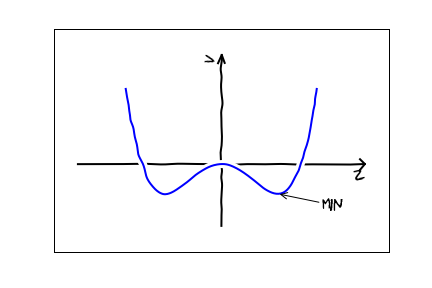
Classically, if you placed the nitrogen in one of those two equilibrium points it would just sit there. Quantum mechanics, however, lets the atom "tunnel" from one minimum to the other. An intuitive picture is that the Heisenberg uncertainty principle says that if you try localize an atom to a precise location, then it will have a large momentum uncertainty. Thus if you pinpoint the atom at the precise minimum, it has enough energy to get over the barrier. On the other hand, if you make the atom so slow that it cannot get over the barrier, its position is so uncertain that it has some probability of being on the other side of the barrier. Mathematically, this is all contained in the Schrodinger equation -- it is not something extra which needs to be added.

We will soon have the tools to start from the Schrodinger equation for $\psi(x)$ and prove that this tunneling occurs. Right now, however, I just want to take for granted that this is the right physics, and see how we can model it.

The first thing to think about is what is the minimal description of this physics. In my mind there are just two numbers we need to know: $\psi_L(t)$ and $\psi_R(t)$. These are the amplitudes for the nitrogen atom to be in the left or right well. So $|\psi_L(t)|^2$ is the probability of being on the left and $|\psi_R(t)|^2$ is the probability of being on the right. Maybe more concretely, my mental picture is
\begin{equation}
\psi(x,t) = \psi_L(t) \phi_L(x) + \psi_R(t) \phi_R(x).
\end{equation}
That is there are two spatial modes:

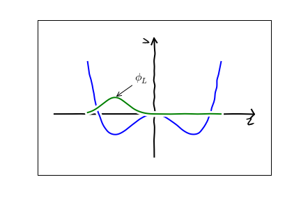
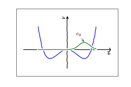
The nitrogen hops between them.

The equations of motion of quantum mechanics are linear, so the most general form that the Schrodinger equation can possibly take here is
\begin{equation}\label{hop}
i\partial_t \left(\begin{array}{c}\psi_L(t)\\\psi_R(t)\end{array}\right)=
\left(\begin{array}{cc}a&b\\ c&d\end{array}\right)\left(\begin{array}{c}\psi_L(t)\\\psi_R(t)\end{array}\right),
\end{equation}
where $a,b,c,d$ are constants. By symmetry we can assume $a=d$ and $b=c$. By this I mean that since the right and left wells are the same, the dynamics should be unchanged if I switch the labels $L$ and $R$. The only way that can be true is if $a=d$ and $b=c$. This is the first example of an important principle we will see over and over in this course: Symmetries constrain the Hamiltonian. We will see that symmetries also play an important role in the distribution of eigenstates of the Hamiltonian.

We want to see than Eq.~(\ref{hop}) has the basic behavior we are after. Suppose at time $t=0$ the nitrogen atom is on the left (so $\psi_L(0)=1$ and $\psi_R(0)=0$) we want to know what is the probability that the particle is on the right at a later time.

Complete the Dynamics Worksheet.

We want to solve the differential equation
\begin{equation}\label{hop2}
i\partial_t \left(\begin{array}{c}\psi_L(t)\\\psi_R(t)\end{array}\right)=
\left(\begin{array}{cc}a&b\\ b&a\end{array}\right)\left(\begin{array}{c}\psi_L(t)\\\psi_R(t)\end{array}\right)
\end{equation}
with initial conditions $\psi_L(0)=1$ and $\psi_R(0)=0$.

There are many ways to solve equations like this. The most easily generalized involves first finding the eigenvectors and eigenvalues of the matrix
\begin{equation}
H=\left(\begin{array}{cc}a&b\\ b&a\end{array}\right).
\end{equation}
Recall that eigenvectors and eigenvalues are solutions to the equations
\begin{equation}\label{hm}
H\left(\begin{array}{c}\psi_L\\\psi_R\end{array}\right)=E\left(\begin{array}{c}\psi_L\\\psi_R\end{array}\right).
\end{equation}
I hate writing out vectors like this, so I will use "kets" to denote column vectors
\begin{equation}
|\psi\rangle=\left(\begin{array}{c}\psi_L\\\psi_R\end{array}\right).
\end{equation}
This is better for us than $\vec \psi$, as the latter connotes a 3D spatial vector.

Some people like to solve eigenvalue problems like Eq.~(\ref{hm}) by finding the roots of the characteristic equation. I prefer to start by guessing the eigenvectors. If there is symmetry to the problem that is faster. Since left and right are equivalent, the natural guesses are
\begin{equation}
|+\rangle=\left(\begin{array}{c}1/\sqrt{2}\\1/\sqrt{2} \end{array}\right),\qquad|-\rangle=\left(\begin{array}{c}1/\sqrt{2}\\-1/\sqrt{2} \end{array}\right).
\end{equation}
I normalized these -- which is convenient, but unnecessary. Plugging these into Eq.~(\ref{hm}) we find that these are indeed eigenvectors, and the
eigenvalues are
\begin{equation}
E_{\pm}= a\pm b.
\end{equation}

The next step is we expand our initial conditions in these vectors, writing
\begin{equation}\label{expansion}
|\psi(t)\rangle=\left(\begin{array}{c}\psi_L(t)\\\psi_R(t)\end{array}\right)= \alpha(t) |+\rangle+ \beta(t) |-\rangle.
\end{equation}
This expansion is unique. One way to see that is to explicitly write out
\begin{equation}
\left(\begin{array}{c}\psi_L(t)\\\psi_R(t)\end{array}\right)= \frac{1}{\sqrt{2}}\left(\begin{array}{cc} 1&1\\1&-1\end{array}\right) \left(\begin{array}{c}\alpha(t)\\\beta(t)\end{array}\right).
\end{equation}
This can be inverted as
\begin{equation}\label{inv}
\left(\begin{array}{c}\alpha(t)\\\beta(t)\end{array}\right) = \frac{1}{\sqrt{2}}\left(\begin{array}{cc} 1&1\\1&-1\end{array}\right) \left(\begin{array}{c}\psi_L(t)\\\psi_R(t)\end{array}\right).
\end{equation}
Thus we have a prescriptive way to go from $\psi_L,\psi_R$ to $\alpha,\beta$ and back. Both directions are unique. Expansions in terms of eigenvectors of Hermitian operators are always unique. In fact, the vectors $|+\rangle$ and $|-\rangle$ are orthogonal, so another way to prove the uniqueness is to take the inner product of Eq.~(\ref{expansion}) with each of these in turn.

We now substitute Eq.~(\ref{expansion}) into Eq.~(\ref{hop}). Using that $|+\rangle$ and $|-\rangle$ are eigenstates, this yields the simple expression
\begin{equation}
i \alpha^\prime(t) |+\rangle+ i \beta^\prime(t) |-\rangle =
E_+ \alpha(t) |+\rangle+ E_-\beta(t) |-\rangle.
\end{equation}
by the uniqueness of the expansion in therm of eigenvectors, we have
\begin{eqnarray}
i\alpha^\prime(t) &=& E_+ \alpha(t)\\
i \beta^\prime(t) &=& E_- \beta(t).
\end{eqnarray}
which are easily integrated as
\begin{eqnarray}
\alpha(t) &=& \alpha(0) e^{-i E_+ t}\\
\beta(t) &=& \beta(0) e^{-i E_- t}.
\end{eqnarray}

Next we need to determine $\alpha(0)$ and $\beta(0)$. From Eq.~(\ref{inv}),
\begin{eqnarray}
\alpha(0) &=& 1/\sqrt{2}\\
\beta(0) &=& 1/\sqrt{2}.
\end{eqnarray}
This yields
\begin{eqnarray}
\left(\begin{array}{c}\psi_L(t)\\\psi_R(t)\end{array}\right) &=& \frac{1}{\sqrt{2}} e^{- i E_+ t} \left(\begin{array}{c}1/\sqrt{2}\\1/\sqrt{2} \end{array}\right)
+ \frac{1}{\sqrt{2} }e^{- i E_- t} \left(\begin{array}{c}1/\sqrt{2}\\-1/\sqrt{2} \end{array}\right).
\end{eqnarray}
In particular
\begin{eqnarray}
\psi_R(t) &=& \frac{e^{- i E_+ t}-e^{- i E_- t}}{2}\\
&=& i e^{-i (E_+ + E_-) t/2} \frac{e^{- i (E_+-E_-) t/2}-e^{- i (E_--E_+) t/2}}{2i}\\
&=& i e^{-i (E_+ + E_-) t/2} \sin\left(\frac{(E_- - E_+) t}{2}\right).
\end{eqnarray}
The probability of being on the right at time $t$ is
\begin{equation}
P_R(t) = |\psi_R(t)|^2 = \sin^2\left(\frac{(E_- - E_+) t}{2}\right)= \sin^2 (b t).
\end{equation}
Thus our model does indeed capture the idea of tunneling.

Beyond the functional form

This argument is typical of what one finds in theoretical physics. One uses symmetries to argue about the allowed structure of the theory. You have some free parameters. You then show that the answer must have some functional form. Our time-of-flight expansion argument was similar. The next question is how do you {\em a-postiori} verify your assumptions, and how do you estimate the parameters.

In the present case, the best route to understanding the parameters is not through the dynamics, but through the energy eigenvalues. The parameter $b$ is the energy splitting between two quantum states, whose wavefunctions look like this:


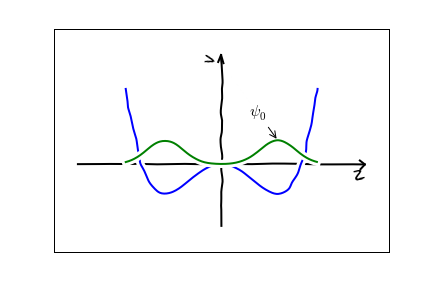
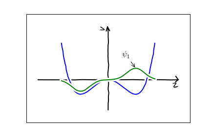
The approximation of truncating our physical space to linear combinations of these two states will make sense if there is a separation of scales, and these two states have much lower energy than all other quantum states. More precisely, if we label the energies of subsequent energy eigenstates as $E_0,E_1,E_2,\cdots$. Our approximations require $|E_1-E_0|\ll E_2$. We refer to this as a near-degeneracy.

In a few lectures we will prove that a double-well potential generically leads to a near-degeneracy, and find a way to estimate the splitting. One interesting thing we will find is that $b$ is always negative. Thus the symmetric state has a lower energy than the antisymmetric.